Welcome

I discovered “An Introduction to Statistical Learning” (ISLR) a few years ago, and since then, it’s become my go-to reference for machine learning. Lately, I’ve been itching to dive deeper into the new edition—especially with the updated chapters, Python labs, and all the fresh content.

Between the book itself, the video lectures available on edX (and other platforms), and the awesome book club run by the DSLC community, I’ve really immersed myself in this world.

It’s been the perfect opportunity to revisit the fundamentals with a fresh, more relaxed mindset. Learning just for the joy of it—rather than to pass a test—is a totally different experience. And honestly, it’s so much more satisfying.

To keep a record of this deep dive, I decided to start a blog. The good news? It’s incredibly easy to set up with Quarto, and hosting it on GitHub is a breeze.

I’m not trying to summarize the book or highlight the key concepts. That’s not the goal. I just want to take the time to explore the parts that speak to me—to reflect, to play, to understand better. Kind of like a personal study journal, but online.

1-Classification

Bayses classifiers

Let us focus on understanding the differences between 3 classifiers : Naive Bayses, Linear Discriminant Analysis, and Quadratic Discriminant Analysis.

• Naive Bayses assume that within the kth class, the p preditors are independent.
• LDA assume that the observations are drawn from a multivariate Gaussian \(X \sim \mathcal{N}(\mu_k, \Sigma)\)
• QDA assume that each class has its own covariance matrix \(X \sim \mathcal{N}(\mu_k, \Sigma_k)\)

Principle: We model the distribution of X in each of the classes separately and then we use Bayses theorem to flip things around to obtain Pr(Y|X). By choice, we use the normal (Gaussian) distribution.

\[ Pr(Y = k \mid X = x) = \frac{\pi_k f_k(x) }{\sum_{l=1}^{K} \pi_l*f_l(x)} \]

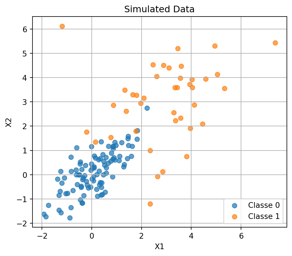
Let us just try on simulated data.

Comparation between “manual” and “sklearn” models

import numpy as np
import pandas as pd
import matplotlib.pyplot as plt
from sklearn.metrics import classification_report

# Fixer le seed pour la reproductibilité
np.random.seed(42)

# 2. Taille des classes
n_0 = 100  # classe majoritaire
n_1 = 40   # classe minoritaire

# 3. Paramètres des distributions
# Classe 0 : petite variance, forte corrélation
mean_0 = [0, 0]
cov_0 = [[1, 0.8], [0.8, 1]]
X0 = np.random.multivariate_normal(mean_0, cov_0, size=n_0)
y0 = np.zeros(n_0)

# Classe 1 : plus grande variance, faible corrélation
mean_1 = [3, 3]
cov_1 = [[2, 0.2], [0.2, 2]]
X1 = np.random.multivariate_normal(mean_1, cov_1, size=n_1)
y1 = np.ones(n_1)

# 4. Fusionner les données
X = np.vstack((X0, X1))
y = np.hstack((y0, y1))

# Mise en DataFrame

# 5. Création du DataFrame
df = pd.DataFrame(X, columns=["X1", "X2"])
df["Y"] = y.astype(int)

from sklearn.preprocessing import StandardScaler
scaler = StandardScaler(with_mean=True,
                        with_std=True,
                        copy=True)
scaler.fit(df[['X1', 'X2']])
X_std = scaler.transform(df[['X1', 'X2']])       

df_scale = pd.DataFrame(
                 X_std,
                 columns=['X1', 'X2'])
df_scale["Y"] = y.astype(int)

# Aperçu des données


# 2. Estimer les paramètres nécessaires

def get_stat(df):
   # Séparer les classes
    df_class0 = df[df['Y'] == 0]
    n_0 = len(df_class0)
    df_class1 = df[df['Y'] == 1]
    n_1 = len(df_class1) 



    # Probabilités a priori
    prior_0 = n_0 / len(df)
    prior_1 = n_1 / len(df)

    # Moyennes et variances (indépendance des features)
    mu_0 = df_class0[['X1', 'X2']].mean()
    var_0 = df_class0[['X1', 'X2']].var()

    mu_1 = df_class1[['X1', 'X2']].mean()
    var_1 = df_class1[['X1', 'X2']].var()


    # Matrices de covariance individuelles
    cov_0 = np.cov(df_class0[['X1', 'X2']].T)
    cov_1 = np.cov(df_class1[['X1', 'X2']].T)
    det_cov_0 = np.linalg.det(cov_0)
    det_cov_1 = np.linalg.det(cov_1)
    inv_cov_0 = np.linalg.inv(cov_0)
    inv_cov_1 = np.linalg.inv(cov_1)
    # Matrice de covariance commune (pooled)
    pooled_cov = ((n_0 - 1) * cov_0 + (n_1 - 1) * cov_1) / (n_0 + n_1 - 2)
    inv_pooled_cov = np.linalg.inv(pooled_cov)
    dict_values ={
        "prior_0": prior_0,
        "prior_1": prior_1,
        "mu_0" :mu_0,
        "mu_1" :mu_1,
        "var_0" :var_0,
        "var_1" :var_1,
        "inv_cov_0": inv_cov_0,
        "inv_cov_1": inv_cov_1,
        "det_cov_0" :det_cov_0,
        "det_cov_1" :det_cov_1,
        "inv_pooled_cov": inv_pooled_cov


    }
    return dict_values




# Fonction de densité gaussienne
def gaussian_pdf(x, mean, var):
    return (1.0 / np.sqrt(2 * np.pi * var)) * np.exp(- ((x - mean) ** 2) / (2 * var))

# 3. Fonction discriminante LDA
def lda_discriminant(x, mu, inv_cov, prior):
    return x @ inv_cov @ mu - 0.5 * mu.T @ inv_cov @ mu + np.log(prior)

# --- QDA : fonction discriminante ---
def qda_discriminant(x, mu, inv_cov, det_cov, prior):
    return -0.5 * np.log(det_cov) - 0.5 * (x - mu).T @ inv_cov @ (x - mu) + np.log(prior)

    
# --- Naive Bayes : prédiction manuelle ---
def predict_naive_bayes(x, stats):
    probs_0 = gaussian_pdf(x, stats["mu_0"].values, stats["var_0"].values)
    probs_1 = gaussian_pdf(x, stats["mu_1"].values, stats["var_1"].values)
    likelihood_0 = np.prod(probs_0) * stats["prior_0"]
    likelihood_1 = np.prod(probs_1) * stats["prior_1"]
    return 0 if likelihood_0 > likelihood_1 else 1

def predict_lda(x, stats):
  
    score_0 = lda_discriminant(x, stats["mu_0"].values, stats["inv_pooled_cov"], stats["prior_0"])
    score_1 = lda_discriminant(x, stats["mu_1"].values, stats["inv_pooled_cov"], stats["prior_1"])
    return 0 if score_0 > score_1 else 1

def predict_qda(x, stats):
    score_0 = qda_discriminant(x, stats["mu_0"], stats["inv_cov_0"], stats["det_cov_0"], stats["prior_0"])
    score_1 = qda_discriminant(x, stats["mu_1"], stats["inv_cov_1"], stats["det_cov_1"], stats["prior_1"])
    return 0 if score_0 > score_1 else 1

# Récupération des observations
X_values = df[['X1', 'X2']].values
X_values_scale = df_scale[['X1', 'X2']].values
from sklearn.metrics import classification_report
from sklearn.naive_bayes import GaussianNB
from sklearn.discriminant_analysis import LinearDiscriminantAnalysis, QuadraticDiscriminantAnalysis
from sklearn.neighbors import KNeighborsClassifier
import statsmodels.api as sm

from sklearn.metrics import classification_report
# Dictionnaire des fonctions de prédiction manuelle
def calcul_accuracy(df):
    X_values = df[['X1', 'X2']].values
    y = df["Y"].values
    stats = get_stat(df)

    # Re-définir les fonctions manuelles en utilisant les stats locales
    manual_models = {
        "Naive Bayes (manual)": lambda x: predict_naive_bayes(x, stats),
        "LDA (manual)": lambda x: predict_lda(x, stats),
        "QDA (manual)": lambda x: predict_qda(x, stats)
    }

    # Inclure aussi les modèles sklearn
    non_manual_models = {
        "Naive Bayes": GaussianNB(),
        "LDA": LinearDiscriminantAnalysis(),
        "QDA": QuadraticDiscriminantAnalysis(),
        "KNN1": KNeighborsClassifier(n_neighbors=1),
        "KNN2": KNeighborsClassifier(n_neighbors=2),
        "KNN3": KNeighborsClassifier(n_neighbors=3),
        "KNN4": KNeighborsClassifier(n_neighbors=4),
        "KNN5": KNeighborsClassifier(n_neighbors=5),
        "GLM (Binomial)": "glm"
    }

    all_accuracies = {}

    # Prédictions manuelles
    for name, predict_func in manual_models.items():
        preds = np.array([predict_func(x) for x in X_values])
        acc = classification_report(y, preds, output_dict=True)["accuracy"]
        all_accuracies[name] = acc

    # Prédictions non manuelles
    for name, model in non_manual_models.items():
        if model == "glm":
            X_glm = sm.add_constant(X_values)
            glm = sm.GLM(y, X_glm, family=sm.families.Binomial())
            glm_result = glm.fit()
            probs = glm_result.predict(X_glm)
            preds = (probs >= 0.5).astype(int)
        else:
            model.fit(X_values, y)
            preds = model.predict(X_values)

        acc = classification_report(y, preds, output_dict=True)["accuracy"]
        all_accuracies[name] = acc

    return all_accuracies
    

# Affichage
#for name, acc in all_accuracies.items():
#    print(f"{name}: {acc:.3f}")

    # Créer un DataFrame pour affichage
accuracy_raw = calcul_accuracy(df)
accuracy_scale = calcul_accuracy(df_scale)

accuracy_df = pd.DataFrame({
    "accuracy_raw": pd.Series(accuracy_raw),
    "accuracy_scale": pd.Series(accuracy_scale)}).round(3)

accuracy_df.index.name = "Model"

📊 Données simulées par classe

plt.figure(figsize=(6, 5))
plt.scatter(df[df.Y == 0]['X1'], df[df.Y == 0]['X2'], label='Classe 0', alpha=0.7)
plt.scatter(df[df.Y == 1]['X1'], df[df.Y == 1]['X2'], label='Classe 1', alpha=0.7)
plt.xlabel("X1")
plt.ylabel("X2")
plt.title("Simulated Data")
plt.legend()
plt.grid(True)
#plt.show()

# Visualisation 2
# Affichage
#print(accuracy_df)
from IPython.display import display, Markdown



# Générer le Markdown avec contrôle CSS
md_table = accuracy_df.to_markdown()

# CSS pour contrôler la largeur des colonnes (via HTML table styling)
style = """
<style>
</style>
"""

# Affichage avec Markdown + style HTML
display(Markdown(md_table))

Model	accuracy_raw	accuracy_scale
Naive Bayes (manual)	0.95	0.95
LDA (manual)	0.936	0.936
QDA (manual)	0.971	0.971
Naive Bayes	0.95	0.95
LDA	0.936	0.936
QDA	0.971	0.971
KNN1	1	1
KNN2	0.971	0.971
KNN3	0.964	0.964
KNN4	0.957	0.957
KNN5	0.957	0.957
GLM (Binomial)	0.943	0.943

Now Let us talk about Fisher discriminant Analysis

# get data
from sklearn.datasets import make_classification
from sklearn.discriminant_analysis import LinearDiscriminantAnalysis
import numpy as np
X,y = make_classification(n_samples = 20, n_features=2,n_classes=2,n_informative=2,n_redundant=0, random_state=42)
model = LinearDiscriminantAnalysis(store_covariance=True, solver='eigen')
model.fit(X,y)
X_single = X[0].reshape(1, -1)

w0 = np.linalg.inv(model.covariance_) @ model.means_[0]
w1 = np.linalg.inv(model.covariance_) @ model.means_[1]

b0 = -0.5 * model.means_[0].T @ w0 + np.log(model.priors_[0])
b1 = -0.5 * model.means_[1].T @ w1 + np.log(model.priors_[1])

z0 = X_single @ w0 + b0
z1 = X_single @ w1 + b1

#
p1 = np.exp(z1) / (np.exp(z1) + np.exp(z0))
p0 = 1 - p1


print("Manual predict_proba :", [p0, p1])
print("sklearn predict_proba:", model.predict_proba(X_single))
print("LDA coef_ :", model.coef_)
# 2. Séparer les classes
X0 = X[y == 0]
X1 = X[y == 1]

# 3. Moyennes
mu0 = X0.mean(axis=0)
mu1 = X1.mean(axis=0)

# 4. Scatter matrices
S0 = (X0 - mu0).T @ (X0 - mu0)
S1 = (X1 - mu1).T @ (X1 - mu1)
S_W = S0 + S1

# 5. Calcul du vecteur de Fisher
w_fisher = np.linalg.inv(S_W) @ (mu1 - mu0)
w_fisher = w_fisher / np.linalg.norm(w_fisher)  # direction normalisée

print("✅ Vecteur de Fisher :", w_fisher)
print("✅ Fisher and coeff are proportionnal", np.isclose(w_fisher[0] / model.coef_[0][0], w_fisher[1] / model.coef_[0][1], 1e-6))

Manual predict_proba : [array([0.93627334]), array([0.06372666])]
sklearn predict_proba: [[0.93627334 0.06372666]]
LDA coef_ : [[-0.56366339  1.76112763]]
✅ Vecteur de Fisher : [-0.30482603  0.95240805]
✅ Fisher and coeff are proportionnal True

# Générer des données 2D avec 3 classes
X, y = make_classification(
    n_samples=150,
    n_features=2,
    n_redundant=0,
    n_informative=2,
    n_clusters_per_class=1,
    n_classes=3,
    random_state=42)
model = LinearDiscriminantAnalysis(store_covariance=True, solver='eigen')
model.fit(X,y)
X_single = X[0].reshape(1, -1)
# On stocke tous les delta_k
deltas = []
for k in range(3):  # ou len(model.classes_)
    mu_k = model.means_[k]
    w_k = np.linalg.inv(model.covariance_) @ mu_k
    b_k = -0.5 * mu_k.T @ w_k + np.log(model.priors_[k])
    delta_k = (X_single @ w_k + b_k).item()
    deltas.append(delta_k)

# Softmax
exp_deltas = np.exp(deltas)
probas = exp_deltas / np.sum(exp_deltas)

print("Manual probas :", probas)
print("sklearn       :", model.predict_proba(X_single)[0])

Manual probas : [7.78108050e-01 2.21523750e-01 3.68200505e-04]
sklearn       : [7.78108050e-01 2.21523750e-01 3.68200505e-04]

data(iris)
library(MASS)
iris.d <- iris[,1:4]  # the data    
iris.c <- iris[,5]    # the classes 
sc_obj <- stepclass(iris.d, iris.c, "lda", start.vars = "Sepal.Width")
sc_obj
plot(sc_obj)

## or using formulas:
sc_obj <- stepclass(Species ~ ., data = iris, method = "qda", 
    start.vars = "Sepal.Width", criterion = "AS")  # same as above 
sc_obj
## now you can say stuff like
## qda(sc_obj$formula, data = B3)